Reading Diffusion Policy, part 1: from formulation to network design

Starting with this post, I'm reading Diffusion Policy: Visuomotor Policy Learning via Action Diffusion by Chi et al., in its extended journal version of the RSS 2023 paper.

In one line: the paper represents a robot's visuomotor policy as a conditional denoising diffusion process. Just as image diffusion denoises noise into an image, Diffusion Policy denoises noise into an action sequence.

I once summarized this paper in a presentation. Looking back at those slides, I'd spent most of them on the front half, the formulation and the network design, so this post keeps the same emphasis. The scope is Section 1 (Introduction), Section 2 (Diffusion Policy Formulation), and Section 3 (Key Design Decisions). The experiments, real-robot results, and limitations (Section 4 onward) are in part 2.

As before, I've noted the spots that confused me and the extra concepts I had to look up. I also generated a couple of illustrations with AI to help; their labels are in Korean.

The problem: policy learning as regression

In the introduction, the authors note that learning a policy from demonstrations can, in its simplest form, be treated as supervised regression from observations to actions:

We have demonstration data, and given the current observation $o$ we train the policy to imitate the expert action $a$. But the paper immediately points out that predicting robot actions differs from other supervised problems:

• Multimodal distributions: in the same state, several different actions can all be correct.
• Sequential correlation: it isn't enough to get one action right; actions over many steps have to be consistent.
• High precision: in manipulation, being slightly off means failing.

The first is especially tricky. Picture pushing a T-shaped block. In some states you can go around the left side of the block, or around the right. Both work. But a plain regression policy can average the two and output something in between, neither left nor right.

Wait: which "multimodal"?

The word multimodal confused me the first time I read this paper. The multimodal I knew meant combining different kinds of data, like camera images, language, and joint states. So I almost skimmed past it thinking, "it's a robot, so it combines camera and joint inputs." It turns out the word has two different meanings:

• Multimodal learning: handling several kinds of input together, such as vision, language, and audio. Here a modality is a type of data.
• Multimodal distribution: a probability distribution with several peaks. Here a mode is a most-frequent value, a point of highest probability.

This paper means the second one. It's not about sensors at all; it's about the shape of the distribution. A unimodal distribution has one peak; a multimodal one has several.

Multimodal action distribution: in a given state, the actions that could be correct form several separate peaks.

There's one peak near "go around the left," another near "go around the right," and a low-probability valley between them. Average the two, and you land right in the valley. That's exactly why a plain regression policy produces a strange in-between action. The paper's Figure 1(a) lists a mixture of Gaussians as one way explicit policies handle multimodality, which is the same idea: mix several Gaussians to get several peaks.

That's enough to follow the rest. But note that in the FiLM section later, "modality" comes back in the first sense, so it's worth keeping the two apart.

Figure 1: three ways to represent a policy

Figure 1 compares three policy representations side by side:

• (a) Explicit policy: feed in an observation and an action comes out directly. Variants differ in how the action is represented: scalar regression, mixture of Gaussians, categorical.
• (b) Implicit policy: feed in the observation and an action, learn a scalar called the energy, and search for the action with the lowest energy.
• (c) Diffusion policy: follow a learned gradient field to refine noise into an action, little by little.

In my slides I'd compressed this into one line each, and it's still the fastest way to see the difference:

(a) Learn the policy. (b) Learn an energy function. (c) Learn the direction in which the score increases.

Energy is not value

One thing about (b) needs care. I wrote "energy function" in my slides, but honestly I was thinking of it like a value function from reinforcement learning, a function that scores actions. I had a reason for the confusion: the two are used almost identically. Both take a state and an action and return one scalar, and both pick actions by that scalar. In RL you choose the action with the highest Q-value; in an implicit policy, the action with the lowest energy. Flip the sign and the usage pattern is basically the same.

The difference is what the scalar measures:

• Value function: the total future reward you expect if you take this action.
• Energy function: how plausible this action is in light of the expert's demonstrations.

That isn't just terminology. This paper assumes behavior cloning from start to finish. There's no reward function anywhere, only the demonstrations a person provided. Without rewards, "the total future reward" doesn't even exist. So the energy here is less a score for actions than a device for defining a probability distribution over actions. The caption of Figure 1 only says that an energy function is learned and the action minimizing the energy landscape is found; nothing about judging how good the action is. And as the equation below shows, the energy sits inside an exponential to form a probability density.

To be fair, there is a formal meeting point: when reinforcement learning is recast as probabilistic inference, energy and value can line up up to a sign and a constant. That comes from a different direction than this post, though, so I'll leave it for later. For now: this paper has no rewards, so the energy isn't a value function.

What Diffusion Policy extracts is, in my words:

Not an estimate of how good a state is, but the direction you should move from it.

For me this is one of the key ideas of Diffusion Policy. It learns a direction, not a value, and that's exactly where it connects to the score functions from the previous paper.

First, a quick look at energy-based policies

In my slides, I put a slide on energy-based policies before getting into the paper, because without it, it's hard to see why the paper keeps saying it's more stable than IBC (Implicit Behavioral Cloning).

An energy-based policy doesn't output an action. It takes an observation $o$ and an action $a$ together and outputs an energy for that pair:

This is Equation (6), from Section 4.4 of the paper. The lower the energy, the more plausible the action. The upside is that multiple action modes are easy to represent: both "go left" and "go right" can get low energy.

The problem is the denominator. The normalizing constant $Z(o,\theta)$ requires integrating over every possible action, which you can't do directly. In practice it's estimated with negative sampling, and the paper says this is exactly what makes training unstable.

(Honestly, I understood maybe half of this the first time, so I took it as written and moved on.)

How Diffusion Policy sidesteps this through the score is derived properly in Equations (7) and (8), in Section 4.4; I cover it in part 2. For now it's enough to know: learning the energy directly is unstable because of $Z$.

Three properties diffusion brings

The introduction lists three properties that come with bringing a diffusion formulation to policies:

• Expressing multimodal action distributions: it learns the gradient of the action score function and samples with stochastic Langevin dynamics, so it can represent almost any normalizable distribution.
• High-dimensional output spaces: diffusion models scale well in high dimensions, as image generation showed, so the policy can infer a whole action sequence at once rather than a single step.
• Stable training: it learns the gradient of the energy rather than the energy itself, so it never has to estimate the normalizing constant.

The third ties straight back to energy-based policies: in the paper's words, it keeps distributional expressivity while gaining training stability. The second isn't just "it scales"; being able to output a whole action sequence at once is directly linked to temporal action consistency, which comes back later.

And three technical contributions

If those properties come for free with diffusion, the paper designs three things itself:

• Closed-loop action sequences: high-dimensional action-sequence prediction combined with receding-horizon control, so the policy keeps replanning while its actions stay temporally consistent.
• Visual conditioning: visual observations are used only as a condition, not as part of the joint distribution, so the visual representation is extracted once regardless of how many denoising iterations run.
• Time-series diffusion transformer: a transformer-based diffusion network that reduces the over-smoothing seen in CNN-based models.

These three are what I consider the most important part of the paper. The earlier properties mostly come with any diffusion model; these are what make it actually work on a real robot.

Section 2.1: DDPM, before it becomes a policy

Section 2 is the Diffusion Policy formulation. The authors first restate a standard DDPM: start from $x_K$ sampled from Gaussian noise and denoise it $K$ times to get $x_0$.

This is Equation (1). The symbols:

• $\epsilon_\theta$: the noise-prediction network being trained (a CNN or a transformer, as we'll see).
• $\gamma$: how much of the predicted noise to subtract.
• $\mathcal{N}(0,\sigma^2 I)$: Gaussian noise added back at every iteration.
• $\alpha$: an overall rescaling. The paper notes that setting it slightly below 1 improves stability.

The paper immediately gives another way to read this:

This is Equation (2). Equation (1) can be seen as one noisy step of gradient descent, where $\epsilon_\theta(x,k)$ effectively predicts the gradient field $\nabla E(x)$ and $\gamma$ acts as a learning rate.

What I found fun here: the paper says choosing $\alpha$, $\gamma$, and $\sigma$ as functions of the iteration $k$, the noise schedule, can be read as learning-rate scheduling in gradient descent. In the earlier posts, I'd only thought of the noise schedule as "how much noise to mix in." Here it reads as "how big a step to take downhill."

Here, $k$ and $t$ are different things

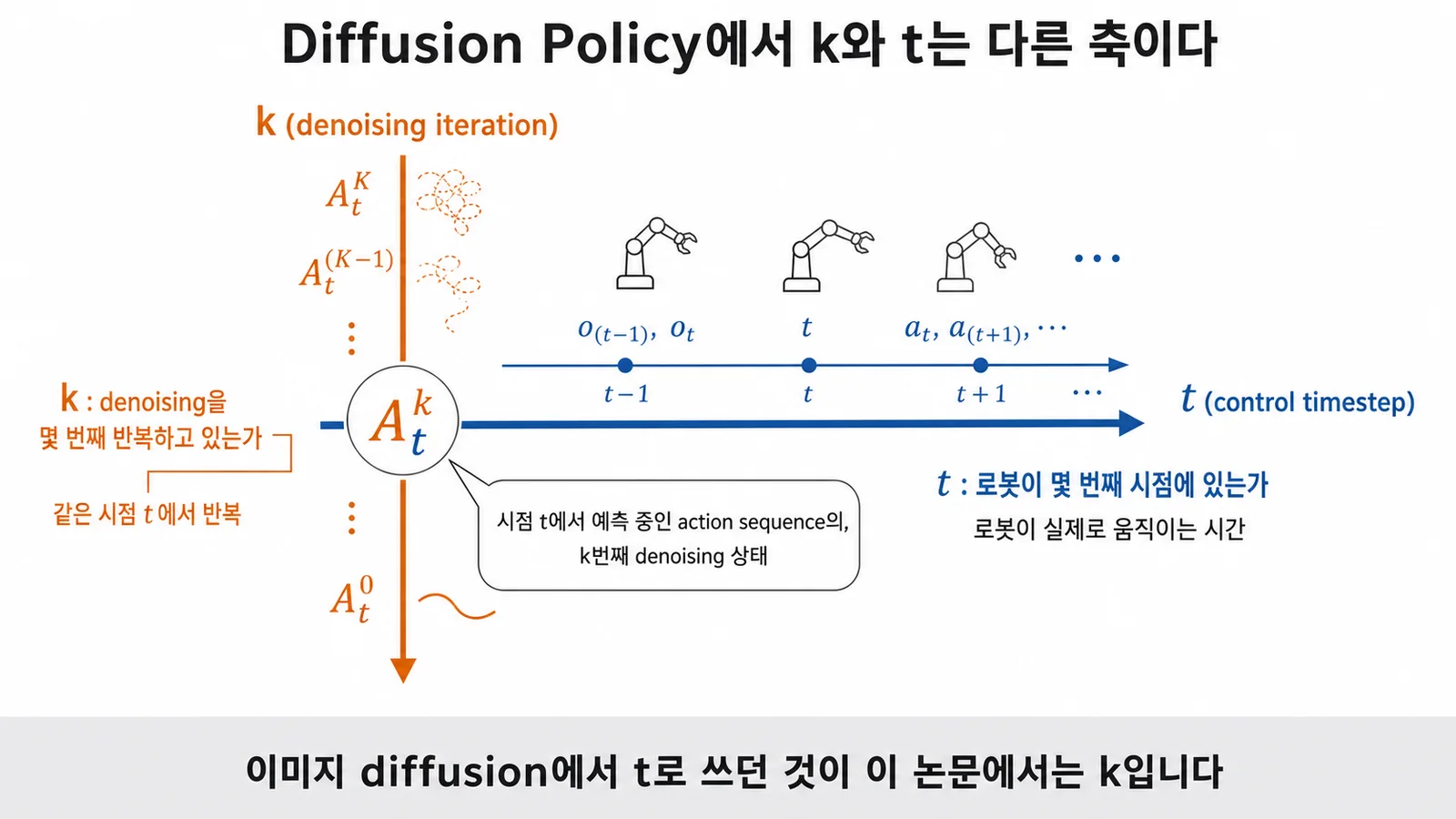
This confused me early on, and it's easy to trip on if you read quickly. Image diffusion usually writes the timestep as $t$, but this paper writes the denoising iteration as $k$. (Think of $k$ as the noising or denoising step carried out at a given point $t$ along the trajectory.) And $t$ means something else entirely: the robot's own time axis, the control timestep.

So a symbol like $A_t^k$, which appears shortly, means "the action sequence being predicted at time $t$, at denoising step $k$." Keep the two apart, and the equations stop looking suddenly complicated.

Section 2.2: DDPM training

Training is almost the same as the noise prediction we saw before. Following the paper: sample an unmodified example $x_0$ from the dataset, pick a denoising iteration $k$ at random, and sample noise $\epsilon_k$ with the variance for that $k$. Then have the network predict that noise from the noised data:

This is Equation (3). The notation is simplified, but it's the familiar DDPM loss: look at the noisy sample and predict the noise that went in. Citing Ho et al., the authors note that minimizing this loss relates to minimizing the variational lower bound of the KL divergence between the data distribution $p(x_0)$ and the distribution $q(x_0)$ the DDPM produces. Yes, it's the same story we spent several posts deriving through the ELBO.

Section 2.3: turning diffusion into a visuomotor policy

Now the key change. To use DDPM as a robot policy, the paper makes two modifications:

• The output $x$ becomes robot actions instead of an image.
• The denoising process is conditioned on the input observation $O_t$.

First, actions. Rather than predicting one step, the policy predicts a sequence, executes part of it, and replans. The paper defines three horizons:

• $T_o$, the observation horizon: how many recent observation steps the policy sees.
• $T_p$, the action prediction horizon: how many future action steps it predicts.
• $T_a$, the action execution horizon: how many of those predicted steps it actually executes.

At time $t$, the policy takes the latest $T_o$ steps of observations $O_t$, predicts $T_p$ steps of actions, and executes $T_a$ of them without replanning. This is receding-horizon control. Predicting a sequence at once improves temporal consistency, but executing too much of it slows the reaction to new observations. The paper also mentions warm-starting the next inference from the previous prediction to make actions smoother.

Second, observation conditioning. The paper states plainly that it approximates the conditional distribution $p(A_t \mid O_t)$, not the joint $p(A_t, O_t)$. So Equation (1) becomes:

This is Equation (4). The important part is the input to $\epsilon_\theta$: the noise-prediction network now sees the observation $O_t$ as well as the noisy action $A_t^k$. It predicts which action noise to remove given this situation. The training loss changes the same way:

This is Equation (5). Add noise to the ground-truth action sequence $A_t^0$, feed it in with the observation $O_t$, and have the model predict the noise $\epsilon_k$. It's exactly what image diffusion did, applied to action sequences, with observations as the condition.

The paper says leaving the observation features out of the denoising output buys two things: faster inference, since it doesn't have to predict future states too; and practical end-to-end training of the vision encoder.

(The paper's Figure 2 lays out the general formulation and both network variants.)

Section 3.1: network architecture, CNN or transformer?

Section 3 covers key design decisions, starting with what network to use for $\epsilon_\theta$. The paper compares two:

• CNN-based Diffusion Policy
• Time-series diffusion transformer

The CNN version takes a 1D temporal CNN and makes three changes:

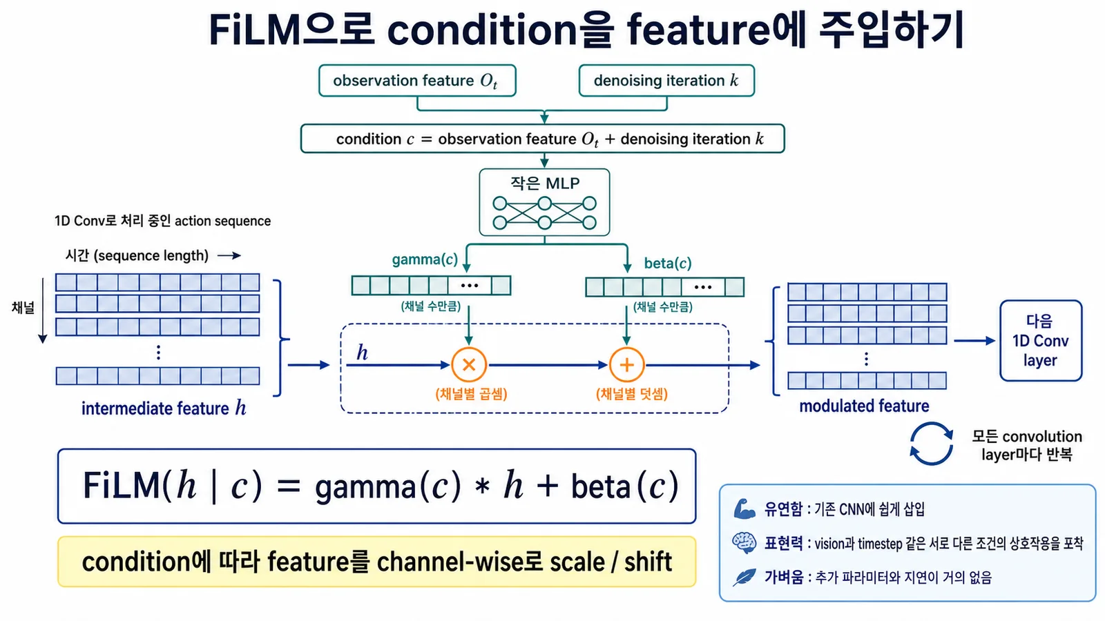
• It conditions on the observation features $O_t$ and the denoising iteration $k$ with FiLM, so it models only the conditional distribution.
• It predicts only the action trajectory, not a trajectory that concatenates observations and actions.
• It drops inpainting-based goal-state conditioning, which doesn't fit the receding prediction horizon.

Figure 2(b) shows FiLM conditioning applied channel-wise at every convolution layer. The paper reports that this CNN backbone worked well on most tasks without much hyperparameter tuning. It also states the limitation clearly: performance drops when the action sequence changes quickly and sharply over time, as with velocity-command action spaces. The reason given is that temporal convolutions have an inductive bias toward low-frequency signals.

That's where the transformer comes in. The noisy actions $A_t^k$ become input tokens to a transformer decoder, with a sinusoidal embedding of the diffusion iteration $k$ prepended as the first token. The observations $O_t$ pass through a shared MLP into an embedding sequence that enters each decoder block through multi-head cross-attention. A causal attention mask lets each action embedding attend only to itself and earlier action tokens.

The paper finds the transformer backbone best on most state-based experiments, especially when the task is complex and actions change quickly, but also more sensitive to hyperparameters. Its practical recommendation:

Start with the CNN version on a new task. If performance falls short because the task is complex or the actions change quickly, then try the transformer.

Wait: what is FiLM?

FiLM is something I had to look up while reading this paper. It stands for feature-wise linear modulation. The idea is simple: given an intermediate feature $h$, compute a scale and a shift from a condition $c$ and use them to modulate the feature.

$c$ is the conditioning input; $\gamma$ and $\beta$ are learned functions. $\gamma(c)$ decides how much to amplify or damp the feature; $\beta(c)$ how much to shift it. In Diffusion Policy, $c$ is the visual observation feature plus the denoising iteration $k$. So as the CNN processes the action sequence, it keeps getting reminded of "what am I looking at" and "which denoising step is this."

In my notes, I'd written down three advantages of FiLM:

• Flexible: it slots fairly easily into an existing CNN.
• Expressive: it captures interactions between different modalities, such as vision and the timestep.
• Lightweight: it adds almost no parameters or latency.

This is the spot I flagged earlier: "modality" in the second bullet is the first meaning, different kinds of input such as visual information and the timestep. It has nothing to do with the peaks of a distribution.

You can also see from its form that it shares the same skeleton as conditional normalization: at the spot where normalization multiplies and adds learned constants, you plug in values computed from the condition instead.

Sections 3.2 to 3.4: the remaining design decisions

Beyond the network, the paper briefly covers choices that matter on a real robot. They're short, but I found them very practical.

Visual encoder. The default is a ResNet-18, trained end-to-end with the diffusion policy and without pretraining. Each camera view gets its own encoder; each timestep's image is encoded separately and the results are concatenated into $O_t$. Two modifications:

• Spatial softmax pooling instead of global average pooling. Position matters in manipulation, and averaging it away would hurt.
• GroupNorm instead of BatchNorm. The paper says this matters when normalization layers are combined with EMA.

The BatchNorm-versus-GroupNorm point didn't click for me at first, so I dug in. BatchNorm contains two different kinds of values:

• Learned parameters: the $\gamma$ and $\beta$ it multiplies and adds after normalizing. These are updated by gradients.
• Running statistics: the mean and variance accumulated over the batches seen during training. These build up independently of gradients and are used for normalization at inference time.

The second kind is the problem. Diffusion models are usually trained with an EMA: a smoothed copy of the weights, updated a little at a time, that is used for inference. It makes training much more stable and results better. But BatchNorm's running statistics were accumulated with the un-averaged weights. So at inference, the weights and the normalization statistics come from different models: we use the averaged weights, but the activation statistics they'd actually produce don't match the stored ones. Small batch sizes, common in robot learning, make it worse, since the mean and variance estimates themselves become noisy.

GroupNorm avoids all of this.

GroupNorm ignores the batch. Within a single sample, it splits the channels into groups and normalizes within each group.

There are no running statistics to remember; mean and variance are computed on the spot from the current input, at training and inference alike. With nothing to fall out of sync, it works fine with EMA and is unaffected by batch size. That's the background to the paper's one-line "for stable training."

Noise schedule. The paper says the noise schedule controls how well the policy captures high- and low-frequency characteristics of the action signal. Empirically, the square cosine schedule from iDDPM worked best.

Faster inference. A policy needs fast inference for closed-loop real-time control. The paper uses DDIM to decouple the number of denoising iterations at training and inference: 100 iterations for training and 10 for inference in the real-robot experiments, for an inference latency of 0.1 s on an Nvidia 3080.

For comparison, when I used Franka and Diffusion Policy as the basis for my own paper, I measured about 184 ms for 64-step inference on an RTX 5070 Ti. The step counts differ by more than six times, so a direct comparison is tricky, but per step it works out to roughly 10 ms for the paper and about 2.9 ms in my setup.

What I took away

Remaking the slides, I felt the first half of the paper boils down to two questions.

The first is what to generate. For images, the target was the image; here, it's an action sequence. And predicting a sequence rather than one step is the key to handling both multimodality and temporal consistency.

The second is what to condition on. Treating observations only as a condition, rather than generating them too, buys both inference speed and end-to-end trainability.

Receding-horizon control, FiLM conditioning, and DDIM acceleration are what make those two decisions work on a real robot.

Summary

This post covered the front half of Diffusion Policy: Visuomotor Policy Learning via Action Diffusion, focusing on the formulation and network design.

• Diffusion Policy represents a robot policy as a conditional denoising diffusion process: given observations $O_t$, it denoises noise into an action sequence $A_t$.
• The ordinary DDPM Equations (1) and (3) become the observation-conditioned Equations (4) and (5), with receding-horizon control and visual conditioning on top.
• Two networks are proposed: a CNN that injects observations with FiLM, and a transformer that injects them with cross-attention.

Personally, the idea of reading the noise schedule as learning-rate scheduling was the freshest part of the paper for me.

In part 2, I move on to Section 4 and beyond: the actual derivation of why Diffusion Policy trains stably, the results across 15 tasks, and the limitations the paper states about itself.