Distributions, Bayes' theorem, expectation, and Jensen's inequality: the four ideas behind the ELBO

This post covers four ideas: distributions, Bayes' theorem, expectation, and Jensen's inequality.

Whenever I learn a basic concept, I want to know why I need it. And my first reaction here was exactly that: why on earth does AI need distributions, expectations, and Bayes' theorem? If you feel the same, this post is my answer.

Distributions

There are many reasons distributions matter, but for generative models four stand out:

• Sometimes the thing we learn is itself a distribution.
• We want the data organized well within a distribution. A generative model can only produce sensible outputs if it samples from a well-organized distribution.
• We want diversity, not a single fixed answer. Classical machine learning maps an input to one fixed output (look at a photo, say "cat"). A generative model should produce a slightly different cat every time, even for the same input. So we interpret the network's output as the parameters of a distribution, such as a mean and a variance, rather than as a fixed value.
• We want control over the output. If we force the latent space into a distribution that is easy to work with, such as a normal distribution, we can later draw a random point from it, like rolling a die, feed it to the decoder, and still get a sensible image.

(The latent space is the space that holds a compressed version of the real data. If "space" feels abstract, just think of it as the compressed data itself.)

To make this concrete, I made an illustration with an image model.

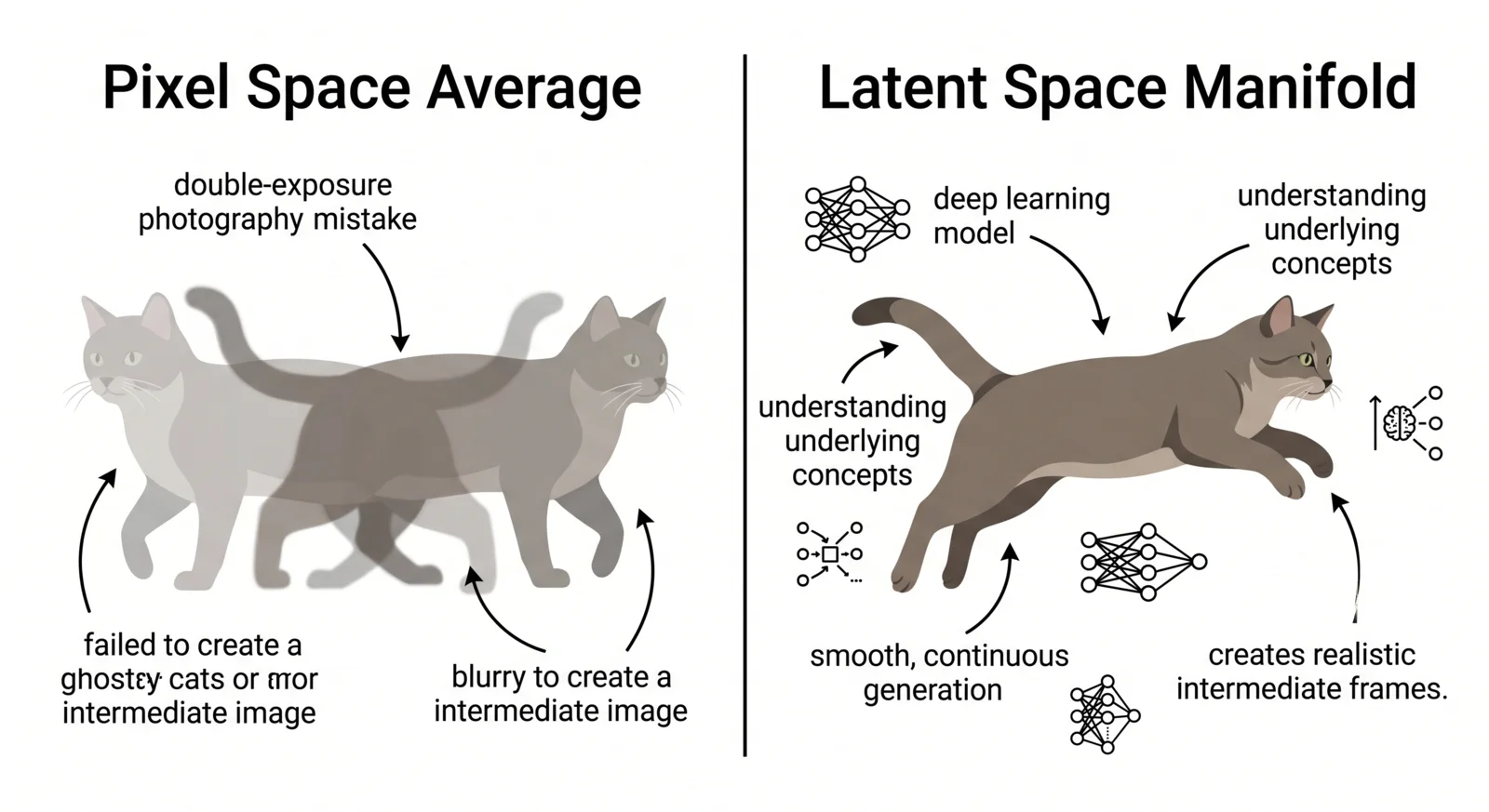
Suppose we have a photo of a cat on the left of the frame (A) and a cat on the right (B). We want the state halfway between them: one cat leaping through the middle of the frame.

• Averaging in pixel space fails. If we simply average A and B in the original high-dimensional space (say $256 \times 256$ pixels), we don't get a new cat in the middle. We get a translucent cat on the left and another on the right, overlapping like a ghostly double exposure. Walking in a straight line between two meaningful points in pixel space leaves the region of natural-looking images (the manifold) and passes through meaningless territory. It's the same reason an interpolated golf swing ends up with four arms and two clubs.
• Averaging in a well-organized latent space works. If the model has learned the low-dimensional manifold where the data actually lives and compresses images onto it, the result is completely different. Take the midpoint between the two cat vectors in latent space and decode it, and the model understands that the midpoint means "halfway in position." It produces one clear cat leaping through the center.

So a generative model has to do more than memorize pixels. It has to learn, and neatly organize, a distribution on which the meaningful changes in the data (position, size, rotation, and so on) vary smoothly and continuously.

Distributions come in two broad kinds, depending on the data:

• Continuous data and the Gaussian distribution. When we predict continuous values such as pixel intensities or coordinates, we assume the output follows a Gaussian (normal, bell-shaped) distribution. If we treat the model's output as the Gaussian's mean $\mu$ and maximize the probability (likelihood) of the data, the terms that remain after dropping constants are exactly the mean squared error (MSE).
• Discrete data and the Bernoulli or categorical distribution. In classification, where the answer is 0 or 1 or one of several classes, we treat the model's outputs as the probabilities of a Bernoulli or categorical distribution. Maximizing the likelihood of the correct answer then leads, somewhat surprisingly, to minimizing the cross-entropy.

The next post derives both.

Bayes' theorem

What is Bayes' theorem, and why do we need it? At first glance it looks like a painfully obvious statement dressed up in notation:

In words: if you see an outcome $B$ and want the probability that $A$ caused it, you have to consider both how plausible $A$ was to begin with and how likely $A$ is to produce $B$.

The four pieces have names:

• $P(A)$, the prior: how plausible $A$ is before seeing $B$.
• $P(B \mid A)$, the likelihood: the probability of observing $B$ if $A$ is the cause.
• $P(A \mid B)$, the posterior: the probability that $A$ was the cause, after observing $B$.
• $P(B)$, the evidence: the overall probability of observing $B$ at all.

At first I didn't see why this mattered for generative models. The key is to read $x$ as the data we observe and $z$ as the hidden cause, or latent variable, that produced it.

Take a handwritten digit image $x$. Some hidden information explains why it looks the way it does: the slant of the digit, the stroke thickness, the handwriting style, its position and rotation. Bundle all of that into $z$. Then the relationships we care about are:

• $p(z)$: what distribution $z$ comes from in the first place.
• $p(x \mid z)$: the probability of generating $x$ given a particular $z$.
• $p(z \mid x)$: given an observed $x$, the probability that a particular $z$ produced it.

The pair that trips people up is $p(x \mid z)$ and $p(z \mid x)$. $p(x \mid z)$ points in the decoder direction: given a latent $z$, produce the data $x$. $p(z \mid x)$ points in the encoder direction: look at the data $x$ and infer the latent $z$ that explains it. Most of the confusing notation in VAEs starts right here.

Rewritten in these terms, Bayes' theorem becomes

In words: to infer which latent $z$ produced an image $x$, we need both whether that $z$ is plausible in the first place and whether that $z$ can actually generate $x$.

We usually set $p(z)$ to a normal distribution that is easy to work with:

This keeps the latent space from scattering in strange ways, so that later we can sample almost any point and still get plausible data. As I said above, a generative model doesn't just predict one correct answer; it creates new data by sampling from a well-organized distribution. Organizing the distribution of $z$ is therefore a big deal.

But there's a problem. What we really want is $p(z \mid x)$, and it's hard to compute directly because of the denominator:

This adds up, over every possible $z$, the probability that $z$ produces $x$. Easy to say, nearly impossible to compute. For high-dimensional data like images, there are far too many possible values of $z$ to integrate over.

So instead of computing $p(z \mid x)$ directly, a VAE introduces a distribution that imitates it:

This $q_\phi(z \mid x)$ is the distribution the encoder learns to approximate. Since the true posterior $p(z \mid x)$ is intractable, we build one a neural network can represent and use it instead. That is the starting point of variational inference, which comes up again later.

Expectation

Next is expectation. It looks like just an average, and that's what I thought too. But next to a probability distribution, it's more accurate to call it a weighted average, where each value is weighted by its probability.

For a discrete random variable:

For a continuous one, the sum becomes an integral:

Each value $x$ contributes in proportion to how likely it is. For a fair die, every face from 1 to 6 is equally likely, so the expectation is an ordinary average. But if some values show up often and others almost never, the frequent values pull the result toward themselves. Expectation is an average that takes the distribution into account.

Why does this matter in deep learning? Because most of the losses we optimize are expectations over some distribution. Cross-entropy, for example (more on it in the next post), can be written as

This averages the model's log-probability $\log q(x)$ under the true data distribution $p$. Put plainly, it checks, on average, whether the model assigns high probability where real data actually occurs.

This surprised me when I first worked through it. Expectation multiplies each value by its weight, right? Look closely at which weight appears here. The quantity we're learning is $\log q(x)$, but it isn't weighted by $q(x)$. It's weighted by $p(x)$, the true probability. In other words, we evaluate the model's log-probability according to how often each value really occurs. This expression will keep coming back, so it's fine to take it on trust for now and come back to its meaning later.

KL divergence is an expectation too:

Measured against the true distribution $p$, it tells us on average how inefficient our model distribution $q$ is.

And the ELBO, which we'll meet soon, is full of expectations like

which means: sample $z$ from $q_\phi(z \mid x)$ and see what the quantity inside comes to on average. Once I started reading expectation as "a way to evaluate something on average over a distribution," the equations that follow felt a lot less intimidating.

Jensen's inequality

Honestly, this one felt the most out of place to me. Distributions, Bayes' theorem, and expectation are at least probability. Why is an inequality suddenly showing up? Because it's the key step in deriving the ELBO.

Jensen's inequality relates two things: applying a function to the average and averaging the function's values. For a convex function $f$:

That is, the function of the average is at most the average of the function. Put a set of points through the function and average the results, and you get at least as much as when you average the points first and then apply the function.

For a concave function such as $\log$, the inequality flips:

This one really matters. When we derive the ELBO, we build a lower bound under $\log p(x)$, a quantity we can't compute directly, and the fact that $\log$ is concave is exactly what makes that possible. So Jensen's inequality is less an abstract inequality than a tool that turns an intractable quantity into a tractable lower bound.

That also explains the name Evidence Lower Bound. The evidence is $p(x)$ from Bayes' theorem. What we really want to maximize is $\log p(x)$: the probability that our model produces the training data. But as we saw, $p(x)$ requires integrating over every latent $z$:

So we can't maximize $\log p(x)$ directly. Instead we build a lower bound we can compute and maximize that. Very roughly:

The right-hand side is the ELBO. You don't need to fully understand it yet. The important point is this:

The ELBO has two parts with two jobs:

• Reconstruction term: makes the model reconstruct the input $x$ well.
• Prior matching term: keeps the distribution of the latent $z$ close to the prior we chose, the normal distribution.

So a VAE isn't just an autoencoder that compresses and reconstructs. It learns to reconstruct well while keeping the latent space in a shape that's convenient to sample from.

This is why I spent so long on organizing distributions at the start. A generative model should give plausible output wherever we sample. For that, the latent space can't be scattered; it has to be as smooth and continuous as possible. VAEs use KL divergence to get there, and diffusion models keep the same distribution-centered view.

Summary

At first these four ideas look unrelated, but from the point of view of generative models they connect naturally:

• A distribution is what a generative model learns and samples from.
• Bayes' theorem links the observed data $x$ to its hidden cause $z$.
• Expectation is how we evaluate a quantity on average over a distribution.
• Jensen's inequality turns an intractable quantity into a tractable lower bound.

Together, they're what you need to understand the VAE's ELBO. In the next post, I'll look at maximum likelihood estimation, cross-entropy, and KL divergence, and show why MSE and cross-entropy aren't arbitrary losses but fall out naturally from probability.