Where MSE and cross-entropy come from: maximum likelihood and KL divergence

This post covers maximum likelihood estimation (MLE), cross-entropy, and KL divergence.

Last time I went on at length about how important distributions are. That leads straight to the next question: how do we actually find a good distribution?

One of the most basic answers is MLE. Once you follow MLE through, the losses we use without thinking in deep learning, like MSE and cross-entropy, stop looking arbitrary. And along the way, cross-entropy and KL divergence turn out to be closely related.

This part confused me at first: lots of equations, and names that all sound alike. I assumed MLE, cross-entropy, and KL divergence were separate topics. They aren't. So let's start with MLE, which is what we ultimately want.

Maximum likelihood estimation

Put simply:

Parameters are the values that pin down a distribution. For a normal distribution, those are the mean $\mu$ and the variance $\sigma^2$ .

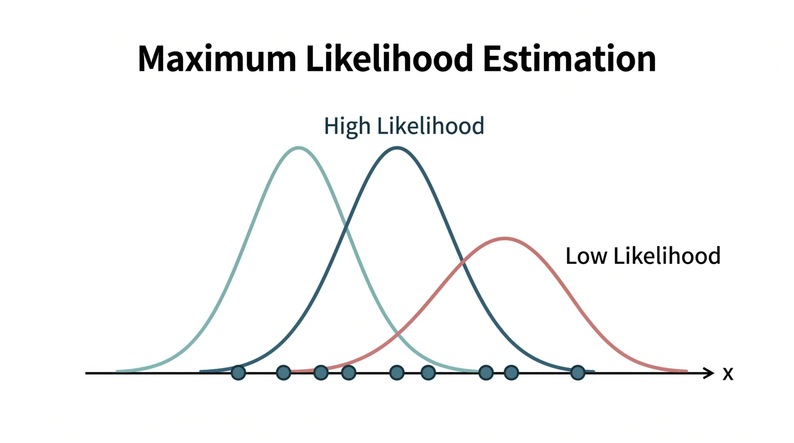
Imagine a scatter of data points. We want to know which distribution they were sampled from. MLE says: find the distribution under which these points were most likely to appear. In other words, find the distribution that best explains the data we already have.

\theta^{*} = \arg\max_\theta\, p_\theta(x_1, x_2, \dots, x_N)

Here $\theta$ is the parameter of the model or distribution, and $p_\theta(x_1, \dots, x_N)$ is the probability of seeing the whole dataset when the parameter is $\theta$ . If we assume the samples are independent, it factors into a product:

p_\theta(x_1, x_2, \dots, x_N)=\prod_{i=1}^{N}p_\theta(x_i)

That product of per-sample probabilities is the likelihood. Probability and likelihood are easy to mix up, so here is the distinction. They look at the same expression from opposite sides:

Probability: the distribution is fixed; how likely is the data?
Likelihood: the data is fixed; how plausible is each parameter setting?

FIG. 1 · Several Gaussian curves over the same data points: the curve centered on the data has high likelihood, the shifted one has low likelihood.

Why take the log?

The likelihood is a product of probabilities:

L(\theta)=\prod_{i=1}^{N}p_\theta(x_i)

Probabilities lie between 0 and 1, and multiplying many such numbers makes the result vanishingly small. That's numerically unstable, and products are awkward to manipulate anyway. So we take the log and work with the log-likelihood:

\log L(\theta)=\log \prod_{i=1}^{N}p_\theta(x_i)=\sum_{i=1}^{N}\log p_\theta(x_i)

The product becomes a sum, which is much easier to handle. And because $\log$ is monotonically increasing, the $\theta$ that maximizes the likelihood also maximizes the log-likelihood. We can swap one problem for the other freely.

Deep learning usually minimizes a loss, so we flip the sign and minimize the negative log-likelihood (NLL):

\theta^{*} = \arg\min_\theta\, -\sum_{i=1}^{N}\log p_\theta(x_i)

Now it looks like an ordinary loss. Minimizing a loss can be read, from the probability side, as maximizing the probability of the data. With that lens, MSE and cross-entropy follow almost immediately.

Continuous data: why a Gaussian gives MSE

Suppose we predict continuous values: pixel intensities, coordinates, noise values. We can treat the model's prediction as the mean of a normal distribution and assume the true value was sampled from it:

y \sim \mathcal{N}(f_\theta(x), \sigma^2)

Here $f_\theta(x)$ is the model's prediction. So the model doesn't hit $y$ exactly; it predicts the mean of the Gaussian that $y$ is likely to come from. The Gaussian density is

p(y \mid x;\theta)=\frac{1}{\sqrt{2\pi\sigma^2}}\exp\left(-\frac{(y-f_\theta(x))^2}{2\sigma^2}\right),

and its negative log-likelihood is

-\log p(y \mid x;\theta)=\frac{(y-f_\theta(x))^2}{2\sigma^2}+\text{constant}.

If $\sigma^2$ is fixed, the only part the model can change is

(y-f_\theta(x))^2,

which should look familiar. It's the mean squared error:

\text{MSE} = \frac{1}{N}\sum_{i=1}^{N}(y_i-\hat{y}_i)^2

So assume a Gaussian, apply MLE, and MSE falls out. That matters, because MSE is easy to memorize as "square the difference and shrink it," but from the probability side it means maximizing the probability that the true value came from the Gaussian the model predicts.

This is also why MSE shows up so often when diffusion models predict noise. Diffusion is built on Gaussian noise, and under certain conditions its noise-prediction objective reduces to an MSE. We'll get there later; for now, remember that MLE under a Gaussian assumption gives MSE.

A spoiler for the next section:

Continuous → Gaussian (normal, bell curve) → MSE
Discrete, categorical → Bernoulli or categorical → cross-entropy

Discrete data: why a categorical distribution gives cross-entropy

Now take a classification problem where the answer is cat, dog, or car. The model outputs a probability for each class, say:

cat: 0.7
dog: 0.2
car: 0.1

If the answer is "cat," the model gave the right class a probability of 0.7. We write the label as a one-hot vector and the model's prediction as a distribution:

y=[1,0,0], \qquad q_\theta=[0.7,0.2,0.1]

Under a categorical distribution, the likelihood of the correct answer is

p(y \mid x;\theta)=\prod_{k=1}^{K}q_\theta(k \mid x)^{y_k}.

This looks odd at first, but the one-hot vector makes it simple. Only the correct class has $y_k = 1$ ; every other exponent is 0, and anything to the power 0 is 1. So only the probability of the correct class survives. Take the negative log:

-\log p(y \mid x;\theta)=-\sum_{k=1}^{K}y_k \log q_\theta(k \mid x)

That's exactly cross-entropy:

H(p,q)=-\sum_x p(x)\log q(x)

Here $p$ is the true distribution and $q$ is the model's. It's the same expression we met last time:

H(p,q)=-E_p[\log q(x)]

In plain terms, it asks how much probability the model gives to the answers that actually occur. Give the right class high probability and $-\log q$ is small; give it low probability and $-\log q$ is large:

-\log(0.9) \approx 0.105, \qquad -\log(0.01) \approx 4.605

So cross-entropy punishes a model hard for putting low probability on the right answer. And, again, it isn't a loss someone invented on a whim:

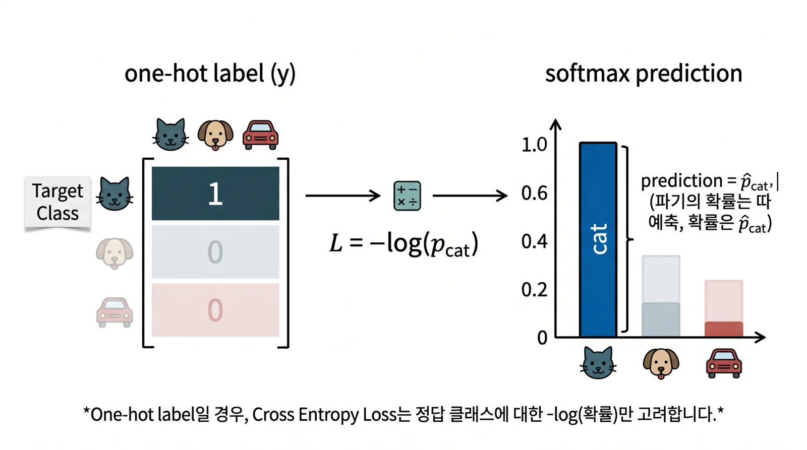
FIG. 2 · Cross-entropy with a one-hot label: only the negative log-probability of the true class counts.

Assume a categorical distribution for discrete data, apply MLE, and cross-entropy comes out naturally.

A point that confused me

Many references define cross-entropy as

H(p,q)=-\sum_x p(x)\log q(x),

but actual deep-learning code often just computes

-\log q(y).

At first I thought these were different formulas. With a one-hot label they're the same: only the true class has $p(x)=1$ , the rest are 0, so only one term survives the sum:

-\sum_x p(x)\log q(x) = -\log q(y)

With label smoothing, where the target isn't strictly one-hot, several terms remain. But for ordinary classification with one-hot labels, cross-entropy is just the negative log-likelihood of the true class.

Entropy, cross-entropy, and KL divergence

Before KL divergence, let's line up entropy and cross-entropy. The three have similar names and similar formulas, which makes them easy to confuse.

Entropy

H(p)=-\sum_x p(x)\log p(x)

is the uncertainty built into the true distribution $p$ itself. A fair coin (0.5 and 0.5) is hard to predict, so its entropy is high. A coin that lands heads 99% of the time is almost predictable, so its entropy is low.

Cross-entropy

H(p,q)=-\sum_x p(x)\log q(x)

is the cost of describing the true distribution $p$ using the model distribution $q$ : how much we lose by believing $q$ when the truth is $p$ .

KL divergence

D_{KL}(p \,\|\, q)=\sum_x p(x)\log\frac{p(x)}{q(x)}

measures how different $p$ and $q$ are. More precisely, it's the extra cost of using $q$ instead of $p$ . Expanding it shows the relationship:

D_{KL}(p \,\|\, q)=\sum_x p(x)\log p(x)-\sum_x p(x)\log q(x) = H(p,q)-H(p)

$H(p)$ is the minimum uncertainty the true distribution carries no matter what. $H(p,q)$ is the total cost of describing $p$ with $q$ . Their difference, the KL divergence, is the extra waste caused by using the predicted distribution instead of the true one.

Personally, I think it's risky to memorize KL divergence as "the distance between two distributions," because it isn't symmetric:

D_{KL}(p \,\|\, q) \neq D_{KL}(q \,\|\, p)

Looking at $q$ from $p$ 's side is different from looking at $p$ from $q$ 's side. Strictly speaking, it's a divergence, not a distance.

Why minimizing cross-entropy is minimizing KL divergence

Some sources say we minimize cross-entropy; others say we minimize KL divergence to bring the model distribution $q$ closer to the true $p$ . How do these connect? Use the same identity:

D_{KL}(p \,\|\, q)=H(p,q)-H(p)

During training we can only change $q$ . The true distribution $p$ is fixed, so $H(p)$ is a constant from the model's point of view. Minimizing $D_{KL}(p \,\|\, q)$ is therefore the same as minimizing $H(p,q)$ .

So minimizing cross-entropy isn't just making a number smaller; it's moving the model's distribution toward the true one. For generative models the goal is the same: make the distribution the model produces match the real data distribution. That's why cross-entropy and KL divergence keep showing up.

Looking at the VAE again

Let's connect this to the VAE. Last time, we roughly wrote the ELBO as

\log p(x) \geq E_{q_\phi(z \mid x)}\left[\log\frac{p_\theta(x,z)}{q_\phi(z \mid x)}\right],

with two jobs: a reconstruction term that makes the model rebuild its input, and a prior matching term that shapes the latent space into the distribution we want.

The reconstruction term pushes $p_\theta(x \mid z)$ up: given a latent $z$ , reconstruct the original $x$ well. If we assume the decoder's output is Gaussian, the reconstruction loss becomes MSE. If we assume Bernoulli or categorical, it becomes binary cross-entropy or cross-entropy. So the VAE's reconstruction loss isn't an arbitrary choice either; it follows from the distribution we assume.

The prior matching term is where KL divergence appears:

D_{KL}(q_\phi(z \mid x)\,\|\,p(z))

It measures how far the encoder's approximate posterior $q_\phi(z \mid x)$ is from the prior $p(z)$ we chose in advance, usually the standard normal:

p(z)=\mathcal{N}(0,I)

So a VAE learns to reconstruct its input while keeping the latent space organized like a standard normal. "Organize the distribution" comes back again: after training, we should be able to sample almost any point in latent space, decode it, and get something plausible. That's impossible if the latent codes are scattered in isolated clumps, so KL divergence keeps $q_\phi(z \mid x)$ from drifting too far from the prior.

The connection to diffusion

Very roughly, a diffusion model gradually adds noise to data until it looks like a standard normal, then generates data by removing that noise step by step. Gaussians are everywhere in that process: the forward process adds Gaussian noise, and the reverse process models Gaussian transitions. So when you read diffusion objectives, likelihood, KL divergence, and MSE keep appearing together.

In particular, from the variational diffusion model point of view we'll meet later, diffusion can be read as a kind of hierarchical VAE. Matching the distributions between timesteps brings in KL divergence, and under Gaussian assumptions part of it reduces to a noise-prediction MSE.

For now, this is enough to take away:

Summary

These terms look like separate topics at first, but they're tightly connected:

MLE finds the distribution parameters that make the observed data most probable.
Maximizing the log-likelihood is the same as minimizing the negative log-likelihood.
Assuming a Gaussian for continuous data makes MLE produce MSE.
Assuming a categorical distribution for discrete data makes MLE produce cross-entropy.
KL divergence is the extra cost of using the predicted distribution instead of the true one.
With the true distribution fixed, minimizing cross-entropy and minimizing KL divergence point the same way.

The losses we use in deep learning aren't empirical hacks; read through probability, they make sense. Once this clicked for me, the losses in VAEs and diffusion models stopped looking like an alien language. It's still not easy material, but I at least got a feel for why each loss is there.

Next, I'll lay out what each of the many probability expressions in VAEs and diffusion models actually means, in a field guide to the notation.