Autoencoders: compression, bottlenecks, and why they aren't quite generative

This post is about the autoencoder (AE).

A note before we start: once you've learned both, the structure of an autoencoder and a diffusion model may look alike. They can look similar, but what they learn, and what that means, is quite different. Keep that in mind as you read, and see if you can spot where they diverge.

In the last post, we went through notation like $x$ , $z$ , $p(x \mid z)$ , and $q_\phi(z \mid x)$ . With autoencoders, the phrase "compress the data and reconstruct it" finally turns into a concrete model.

You need autoencoders before VAEs. A VAE is, after all, a variational autoencoder: an autoencoder with a probabilistic view layered on top. So this post covers what an autoencoder is, why the bottleneck matters, what the reconstruction loss means, and why an autoencoder alone makes a poor generative model.

The goal

Notably, it needs no separate labels. A classifier needs a "cat" label for each cat photo. An autoencoder's target is its own input $x$ :

x \rightarrow \text{AutoEncoder} \rightarrow \hat{x}

$\hat{x}$ is the reconstruction, and training makes $x$ and $\hat{x}$ as close as possible. Your first thought might be: "Can't it just copy the input to the output?" Exactly. That's why the most important part of an autoencoder is the bottleneck.

Structure

An autoencoder has two parts:

Encoder: compresses the input $x$ into a latent representation $z$ .
Decoder: reconstructs $\hat{x}$ from $z$ .

z=f_\theta(x), \qquad \hat{x}=g_\phi(z)

$f_\theta$ is the encoder, $g_\phi$ the decoder, and $z$ the latent vector or latent representation. In the last post I described $z$ as the hidden information that explains the data. In an autoencoder, the encoder looks at $x$ and packs into $z$ whatever the decoder needs to rebuild it.

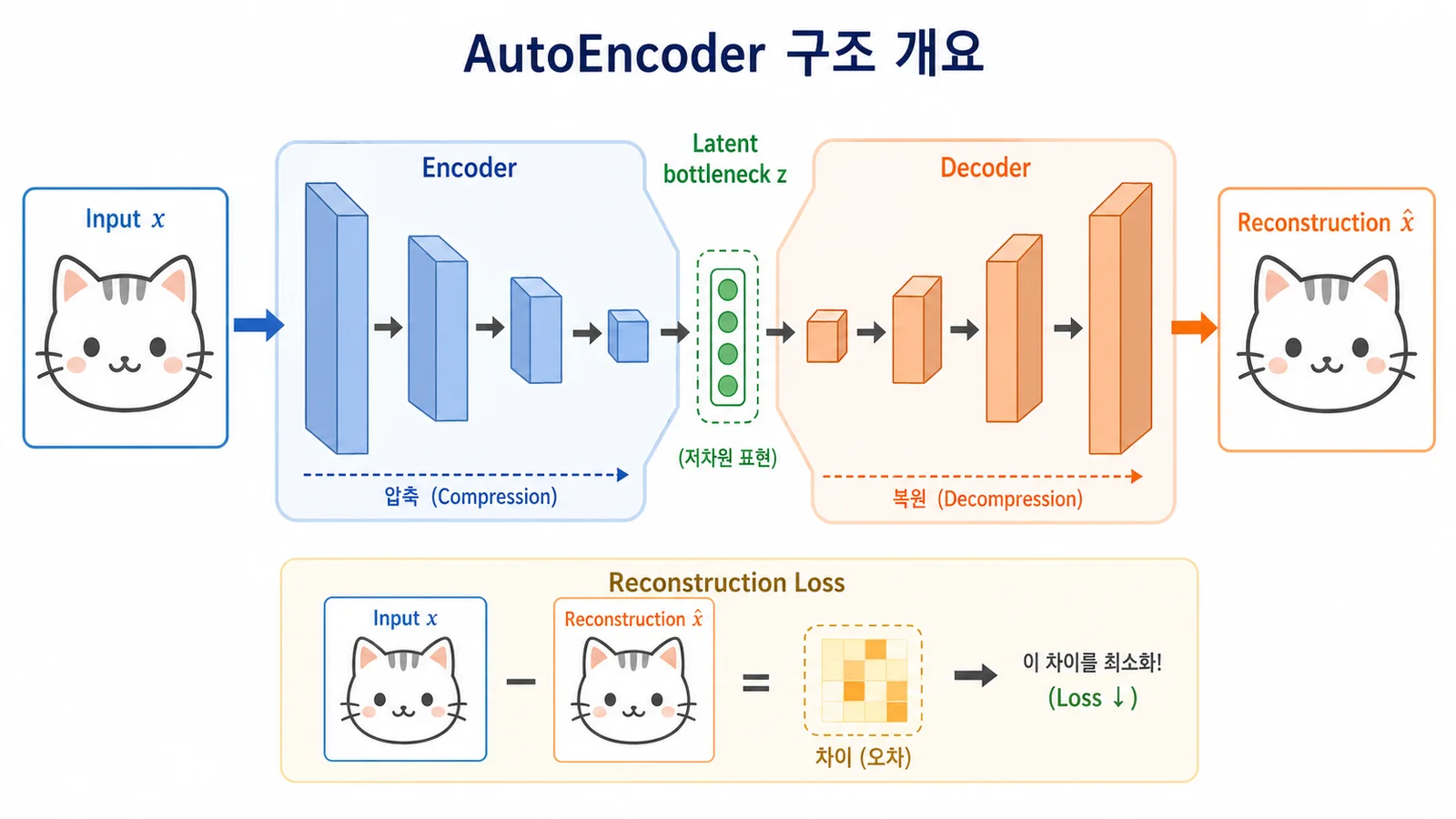
FIG. 1 · Autoencoder structure: the encoder compresses the input into a latent bottleneck, the decoder reconstructs it, and the reconstruction loss compares the two (some labels in Korean).

If $z$ is smaller than the input, the model can't copy every detail. It has to keep only what matters most for reconstruction. That is the heart of the autoencoder.

Why the bottleneck matters

Think of the bottleneck as a narrow passage the data has to squeeze through. An MNIST digit is $28 \times 28$ pixels; flattened, that's a 784-dimensional vector:

28 \times 28 = 784

If the encoder compresses those 784 numbers into a 32-dimensional latent vector, the model can't store them as they are. It has to choose the information that matters for rebuilding the digit, such as:

which digit it is
whether the strokes are thick or thin
whether it leans left or right
whether it's centered
whether the handwriting is round or angular

The bottleneck stops the model from memorizing pixel-level detail and forces it to learn the essential features. Without one, say with a hidden layer larger than the input and no other constraint, the model could learn something close to the identity function. Reconstruction would be excellent, but we wouldn't have learned a meaningful compressed representation. So what matters is not just reconstructing well, but using some constraint to make the representation meaningful.

As you read on, keep asking why learning a representation matters, and why the compress-then-reconstruct loop exists at all.

Reconstruction loss

The autoencoder is trained so that $x$ and $\hat{x}$ match. The loss for that is the reconstruction loss, most simply the MSE:

\mathcal{L}_{\text{rec}}=\|x-\hat{x}\|^2

If pixel values are continuous, MSE is natural. As we saw in part 3, assuming a Gaussian and applying MLE gives exactly MSE. So you can read the reconstruction loss as "shrink the difference," or, probabilistically, as increasing the likelihood of the original input under the distribution the decoder produces.

If we instead treat pixels as near 0 or 1 under a Bernoulli distribution, binary cross-entropy fits. The reconstruction loss depends on the data and the output distribution we assume. The same holds for VAEs, whose reconstruction term also pushes up $p_\theta(x \mid z)$ .

What does an autoencoder learn?

It learns more than a way to compress images. More precisely, it learns a representation from which the input can be rebuilt. To reconstruct a handwritten 7, the model tries to store "this looks like a 7," "the stroke leans right," "the top bar is long," rather than memorizing each pixel.

We can't claim the network stores these as neatly separated, human-readable features. But the idea that a bottleneck forces it to learn a compressed representation needed for reconstruction is central to understanding autoencoders.

That's why autoencoders have long been used for dimensionality reduction, feature extraction, and anomaly detection, with dimensionality reduction and representation learning as the main uses. For anomaly detection: train on normal data only, and the model rebuilds normal data well but struggles with unusual inputs. A large reconstruction error then suggests the input lies off the normal distribution. An autoencoder looks like it just echoes its input, but along the way it learns something about the structure of the data.

Denoising autoencoders

If you're heading toward diffusion, denoising autoencoders deserve a quick look. A denoising autoencoder deliberately corrupts its input with noise and learns to recover the clean original. A plain autoencoder learns

x \rightarrow \hat{x},

while a denoising autoencoder learns

\tilde{x} \rightarrow \hat{x} \approx x,

where $\tilde{x}$ is the noisy input. It sees a dirty input and has to restore the clean one.

That connects intuitively to diffusion, which also learns to remove noise from a noisy image and recover a clean one. Of course, a diffusion model isn't a single denoising autoencoder: it adds noise over many small steps and learns to reverse each one. But the core feel, "recover the original data from a noisy input," is shared. Understanding autoencoders makes diffusion's denoising view feel much less foreign.

Is an autoencoder a generative model?

This is the key question, and the answer is: sort of. An autoencoder compresses and reconstructs, so in one sense it has a decoder that produces data. But nothing guarantees that its latent space is organized for sampling.

Suppose the training data lands in scattered clumps in latent space. Decode a $z$ near a training example and you may get a plausible image. Pick a $z$ at random, though, and it may fall in an empty region where no training data lives, and the decoder can produce something strange. An autoencoder can reconstruct well while its latent space is still poorly organized for generating new samples.

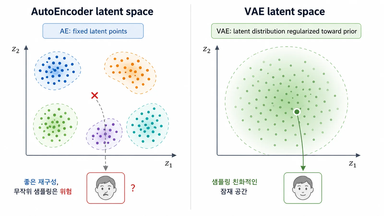
FIG. 2 · Left: an autoencoder's latent space has isolated clusters, so random samples can land in empty regions. Right: a VAE's latent space is regularized toward a prior, making it friendlier to sample (some labels in Korean).

This is where the VAE comes in. A VAE compresses and reconstructs like an autoencoder, but constrains the latent space to follow a distribution that's easy to work with. It usually sets the prior to a standard normal and uses KL divergence to keep the encoder's latent distribution from drifting too far from it. That brings the VAE much closer to a true generative model. The question that takes us from AE to VAE is:

The VAE is the answer.

Connecting AE, VAE, and diffusion

An autoencoder compresses the input into a latent vector and reconstructs it.
A VAE adds a probabilistic view: instead of a single latent vector, it learns the distribution the latent variable follows.
A diffusion model approaches generation differently. Rather than compressing to a latent vector and back in one shot, it learns to add noise gradually and then remove it gradually.

Model	Core idea	As a generator
AE	Compress and reconstruct the input	Weak guarantee that the latent space is good to sample from
VAE	Learn the distribution of the latent variable	Can generate new data by sampling the prior
Diffusion	Learn to add and remove noise	Generates data starting from pure noise

Seen this way, the autoencoder is an important starting point for generative modeling. Compressed representations, reconstruction, and latent spaces keep coming back in VAEs and diffusion. Rather than dismissing autoencoders as an old model, it's worth treating them as the basic structure on the way to VAEs and diffusion.

Summary

An autoencoder compresses its input into a latent vector with an encoder and reconstructs it with a decoder.
The bottleneck keeps the model from copying its input and pushes it to learn the core representation needed for reconstruction.
The reconstruction loss shrinks the input–output gap; probabilistically, it raises the likelihood that the decoder produces the original input.
A plain autoencoder has no guarantee that its latent space is organized for sampling. That limits it as a generative model, and the VAE fixes it with a latent distribution and KL divergence: a standard-normal prior that makes the latent space easy to sample.

Next, we get into the VAE and the ELBO properly.

Once you've read this far, I highly recommend going back to Hwalseok Lee's lecture, Everything about autoencoders (in Korean). It's about three hours, and a great way to consolidate.