What each probability actually means: a field guide to VAE and diffusion notation

So far we've covered distributions, Bayes' theorem, MLE, cross-entropy, and KL divergence. Move on to VAEs or diffusion models, and suddenly the page fills with probability expressions:

$p(x)$, $p(z)$, $p(x \mid z)$, $p(z \mid x)$, $q_\phi(z \mid x)$, $q(x_t \mid x_{t-1})$, $p_\theta(x_{t-1} \mid x_t)$...

My first reaction was: what are all these? What confused me more than any derivation was what each probability actually meant. So this post skips the derivations and goes through each expression with concrete examples.

I also made a one-page summary image with ChatGPT's image generator. It's worth a look before you read on (the labels are in Korean, but the layout follows this post).

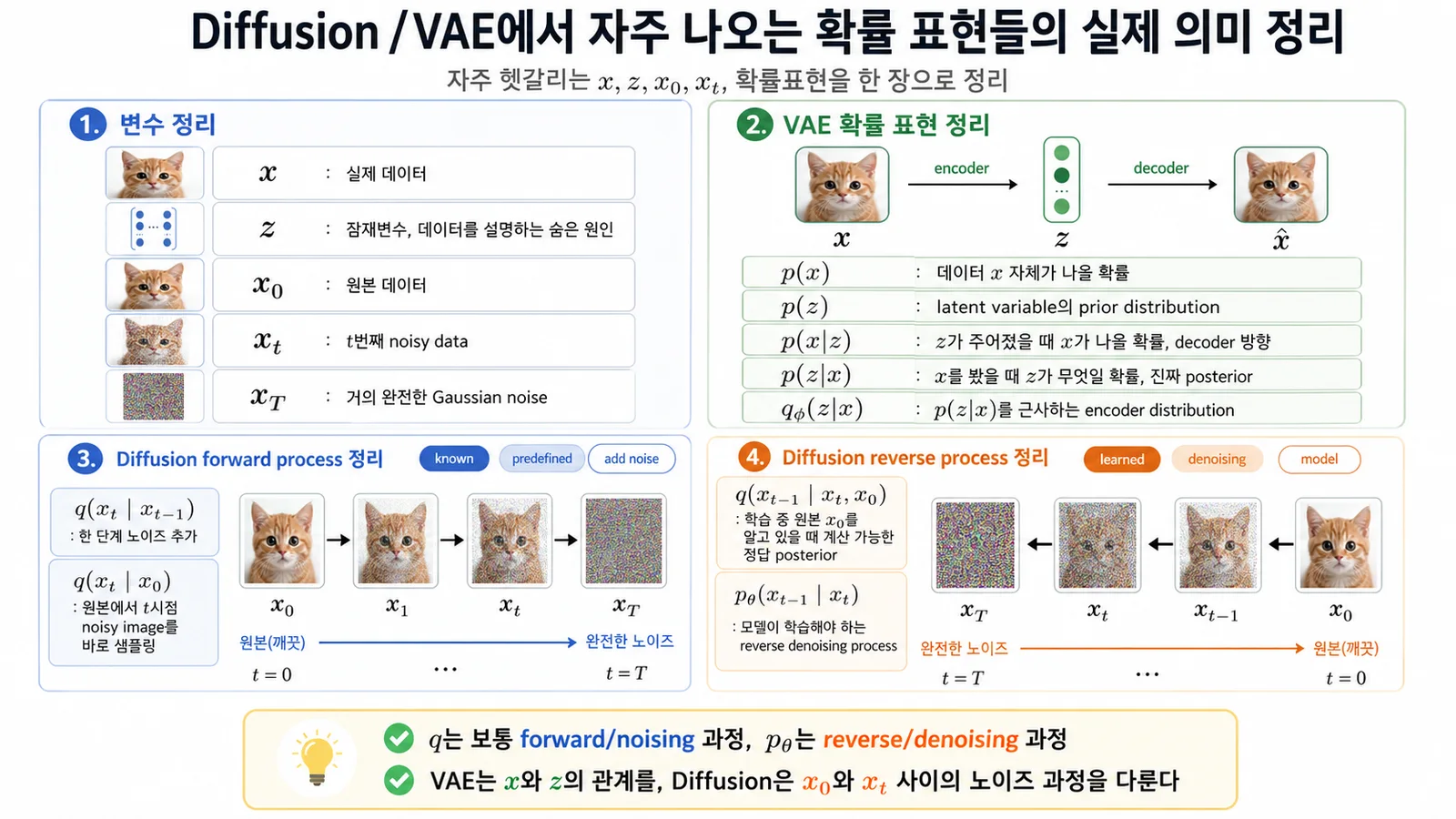
First, what are $x$, $z$, and $x_t$?

Before the probabilities, let's meet the cast. Generative models mostly talk about $x$ and $z$; diffusion adds $x_t$.

VAEs mostly look at the relationship between $x$ and $z$. Diffusion models look at $x_0, x_1, x_2, \dots, x_T$: the same data with more and more noise over time. In short:

Keep that picture in mind and the probabilities get much less confusing.

$p(x)$: how probable the data itself is

$p(x)$ is the probability of the data $x$. For a generative model, it's the thing we ultimately want to know.

If $x$ is a cat photo, $p(x)$ asks how plausible this photo is under the real distribution of images. A well-taken cat photo sits squarely on that distribution. An image of a cat with seven eyes and twisted legs should get a very low probability.

Training a generative model means making the model's distribution match the real data distribution $p_{\text{data}}(x)$. The big goal is: make realistic $x$ have high probability.

The catch is that $p(x)$ is hard to compute directly. VAEs work around it with the ELBO; diffusion models work around it with a multi-step probabilistic process.

$p(z)$: how plausible a hidden cause is to begin with

$p(z)$ is the prior over the latent variable $z$: what we assume about $z$ before seeing any data. VAEs usually make it a standard normal:

Why? To make sampling easy later. After training, a generative model has to make new data, which means we should be able to pick almost any $z$, feed it to the decoder, and get a plausible $x$. If the latent space is scattered in strange ways, we won't know where to sample. So we encourage $z$ to be organized like a standard normal.

For handwritten digits, $z$ might hold stroke thickness, slant, and position. $p(z)$ decides what overall distribution this hidden information should come from.

$p(x \mid z)$: the probability of $x$ given $z$

$p(x \mid z)$ is the probability of $x$ when $z$ is given. In a VAE, think of it as the decoder direction: look at a latent $z$ and produce the data $x$.

Suppose $z$ contains:

• The digit is 7.
• It leans slightly to the right.
• The strokes are thin.
• There's a small hook at the top.

Then $p(x \mid z)$ is the probability of a handwritten 7 that matches this description. A high $p(x \mid z)$ means $z$ explains $x$ well. The VAE's reconstruction term pushes this value up: given $z$, reconstruct the original $x$ well.

$p(z \mid x)$: seeing $x$, which $z$ caused it?

$p(z \mid x)$ is the probability that a particular $z$ produced the $x$ we're looking at. This is the encoder direction.

Look at a handwritten digit and you might say: "That's a 7, it leans right, and the strokes are thin." Those judgments are the hidden information $z$. So $p(z \mid x)$ infers the hidden causes backward from the image. In Bayes' form:

The meaning is intuitive. For a $z$ to be plausible, two things must hold: $z$ itself shouldn't be strange under the prior, $p(z)$; and $z$ should actually produce $x$ well, $p(x \mid z)$.

The problem is that $p(z \mid x)$ is hard to compute, mainly because $p(x)$ in the denominator has to account for every possible $z$. So a VAE doesn't use this true posterior directly; it uses an approximation.

$q_\phi(z \mid x)$: the encoder that approximates $p(z \mid x)$

$q_\phi(z \mid x)$ is central to VAEs. Since the true posterior is intractable, we approximate it with a neural network; $\phi$ are the encoder's parameters. The encoder looks at $x$ and estimates: "this probably came from a $z$ like this."

Importantly, $q_\phi(z \mid x)$ outputs a distribution, not a single value. It usually predicts a mean and a variance:

So even for one image $x$, the candidates for the $z$ that could explain it are expressed as a distribution. For me, this is where a VAE starts to feel genuinely different from an autoencoder. An autoencoder compresses its input into one vector and rebuilds it; a VAE learns the distribution of latent variables that explain its input.

In diffusion, $q$ is usually the forward process

Diffusion papers use $q$ and $p_\theta$ constantly. By convention, $q$ is the forward process: the process that adds noise.

This is the probability of $x_t$ given $x_{t-1}$. In words: if we add a little more noise to the previous image, what does the next one look like?

If $x_0$ is a clean cat photo, $x_1$ has a tiny bit of noise, $x_2$ a bit more, and after enough steps $x_T$ is almost pure noise. The forward process is a Gaussian process we fix in advance. It isn't learned; it's a noising procedure we design. So in diffusion, $q$ is usually the process we already know.

$q(x_t \mid x_0)$: jumping straight from the original to step $t$

You'll also see

the probability of the noisy image $x_t$ given the original $x_0$. Where $q(x_t \mid x_{t-1})$ takes one step at a time, $q(x_t \mid x_0)$ jumps from the original to step $t$ in one go.

Suppose we need to add noise 100 times. $q(x_t \mid x_{t-1})$ adds it once per step. $q(x_t \mid x_0)$ takes the clean photo and directly samples a version noised to step $t$.

This matters because noising step by step from 1 to $t$ every training iteration would be wasteful. Thanks to properties of the Gaussian, we can sample $x_t$ directly from $x_0$. That's what lets diffusion training pick a random $t$ and noise $x_0$ to that level in a single shot.

$p_\theta(x_{t-1} \mid x_t)$: the model that learns to denoise

Now the most important direction. Generation in a diffusion model starts from noise and ends at an image: from $x_T$ back through $x_{T-1}, x_{T-2}, \dots, x_0$. That uses

the probability of the slightly cleaner image $x_{t-1}$ given the current $x_t$:

Unlike the forward process, we don't know this one. Adding noise is easy; removing it is hard. So a neural network has to learn the reverse process, and $\theta$ are its parameters. Whenever you see $p_\theta$ in a diffusion paper, it's usually safe to read it as the reverse, generative process the model learns.

$q(x_{t-1} \mid x_t, x_0)$: the reverse step we can only compute during training

One more expression tends to confuse:

This is the distribution of $x_{t-1}$ when we know both $x_t$ and the original $x_0$. It looks a lot like $p_\theta(x_{t-1} \mid x_t)$, but there's a difference.

$p_\theta(x_{t-1} \mid x_t)$ is what we actually use at generation time, when we don't know $x_0$. $q(x_{t-1} \mid x_t, x_0)$ is a posterior we can compute during training, because then we do have $x_0$. We have the original image, we noised it into $x_t$ ourselves, so we can work out what distribution the intermediate $x_{t-1}$ should follow. The model $p_\theta(x_{t-1} \mid x_t)$ is trained to match that answer.

Very roughly, diffusion training is: make the $p_\theta$ we'll use at generation time imitate the reverse posterior of $q$ that we can compute during training.

Telling $q$ and $p_\theta$ apart

At this point $q$ and $p$ blur together, so here's the diffusion version in one table:

The forward process is designed, so we know it. The reverse process is unknown, so we learn it. And during training we know $x_0$, so we can give the model a target to follow. Diffusion looks complicated mostly because these three are constantly mixed together in the equations.

One example, start to finish

Let's walk through a single cat photo. $x_0$ is the clean photo.

In the forward process, noise is added bit by bit. $q(x_1 \mid x_0)$ adds a tiny bit to make $x_1$; $q(x_2 \mid x_1)$ adds a bit more to make $x_2$. Keep going, and $x_T$ is noise in which you can't tell whether there was ever a cat.

Generation runs the other way. Draw a noise sample $x_T$. The model applies $p_\theta(x_{T-1} \mid x_T)$ to remove a little noise, then $p_\theta(x_{T-2} \mid x_{T-1})$ to remove a little more. Repeat, and you end up with an image close to $x_0$.

So generation in a diffusion model is: start from pure noise and follow the learned reverse process, restoring the image a little at a time. That's why $p_\theta(x_{t-1} \mid x_t)$ matters so much. At every step, the model answers one question: "what does this image look like with a little less noise?"

Quick reference

• $p(x)$: the probability of the data. What a generative model ultimately wants to model well.
• $p(z)$: the prior on the latent variable, usually a standard normal so it's easy to sample.
• $p(x \mid z)$: the probability of $x$ given $z$. The decoder direction.
• $p(z \mid x)$: the probability of $z$ given $x$. The true posterior, but intractable.
• $q_\phi(z \mid x)$: the encoder distribution that approximates $p(z \mid x)$.
• $q(x_t \mid x_{t-1})$: the diffusion forward process. One step of added noise.
• $q(x_t \mid x_0)$: sample the step-$t$ noisy image straight from the original.
• $q(x_{t-1} \mid x_t, x_0)$: the correct reverse posterior, computable during training.
• $p_\theta(x_{t-1} \mid x_t)$: the reverse denoising process the model learns.

There's a lot of notation, but it boils down to a few questions:

• Does this probability point in the direction of generating data, or of inferring causes from data?
• In diffusion, does it add noise or remove noise?
• Is it a process we already know, or one we have to learn?

With those questions in hand, you can keep your bearings even when the equations get messier. Next, we get into model structure properly, starting with autoencoders.